An S4 Class implementing the Isomap Algorithm
Details
The Isomap algorithm approximates a manifold using geodesic distances on a k nearest neighbor graph. Then classical scaling is performed on the resulting distance matrix.
Slots
funA function that does the embedding and returns a dimRedResult object.
stdparsThe standard parameters for the function.
General usage
Dimensionality reduction methods are S4 Classes that either be used
directly, in which case they have to be initialized and a full
list with parameters has to be handed to the @fun()
slot, or the method name be passed to the embed function and
parameters can be given to the ..., in which case
missing parameters will be replaced by the ones in the
@stdpars.
Parameters
Isomap can take the following parameters:
- knn
The number of nearest neighbors in the graph. Defaults to 50.
- ndim
The number of embedding dimensions, defaults to 2.
- get_geod
Should the geodesic distance matrix be kept, if
TRUE, access it asgetOtherData(x)$geod
Implementation
The dimRed package uses its own implementation of Isomap which also
comes with an out of sample extension (known as landmark
Isomap). The default Isomap algorithm scales computationally not
very well, the implementation here uses nn2 for
a faster search of the nearest neighbors. If data are too large it
may be useful to fit a subsample of the data and use the
out-of-sample extension for the other points.
References
Tenenbaum, J.B., Silva, V. de, Langford, J.C., 2000. A Global Geometric Framework for Nonlinear Dimensionality Reduction. Science 290, 2319-2323. https://doi.org/10.1126/science.290.5500.2319
See also
Other dimensionality reduction methods:
DRR-class,
DiffusionMaps-class,
DrL-class,
FastICA-class,
FruchtermanReingold-class,
HLLE-class,
KamadaKawai-class,
MDS-class,
NNMF-class,
PCA-class,
PCA_L1-class,
UMAP-class,
dimRedMethod-class,
dimRedMethodList(),
kPCA-class,
nMDS-class,
tSNE-class
Examples
if(requireNamespace(c("RSpectra", "igraph", "RANN"), quietly = TRUE)) {

dat <- loadDataSet("3D S Curve", n = 500)
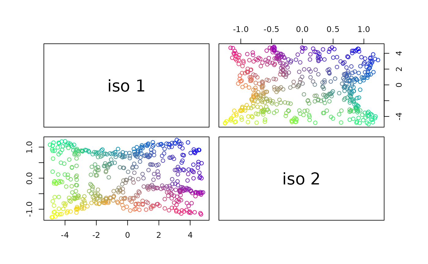
emb <- embed(dat, "Isomap", knn = 10)
plot(emb)

## or simpler, use embed():
samp <- sample(nrow(dat), size = 200)
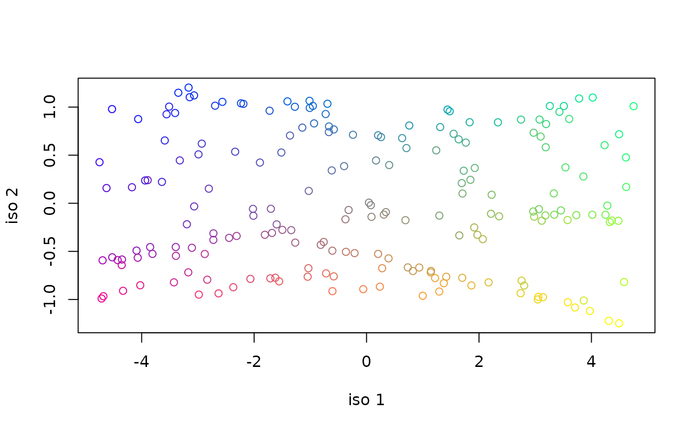
emb2 <- embed(dat[samp], "Isomap", .mute = NULL, knn = 10)
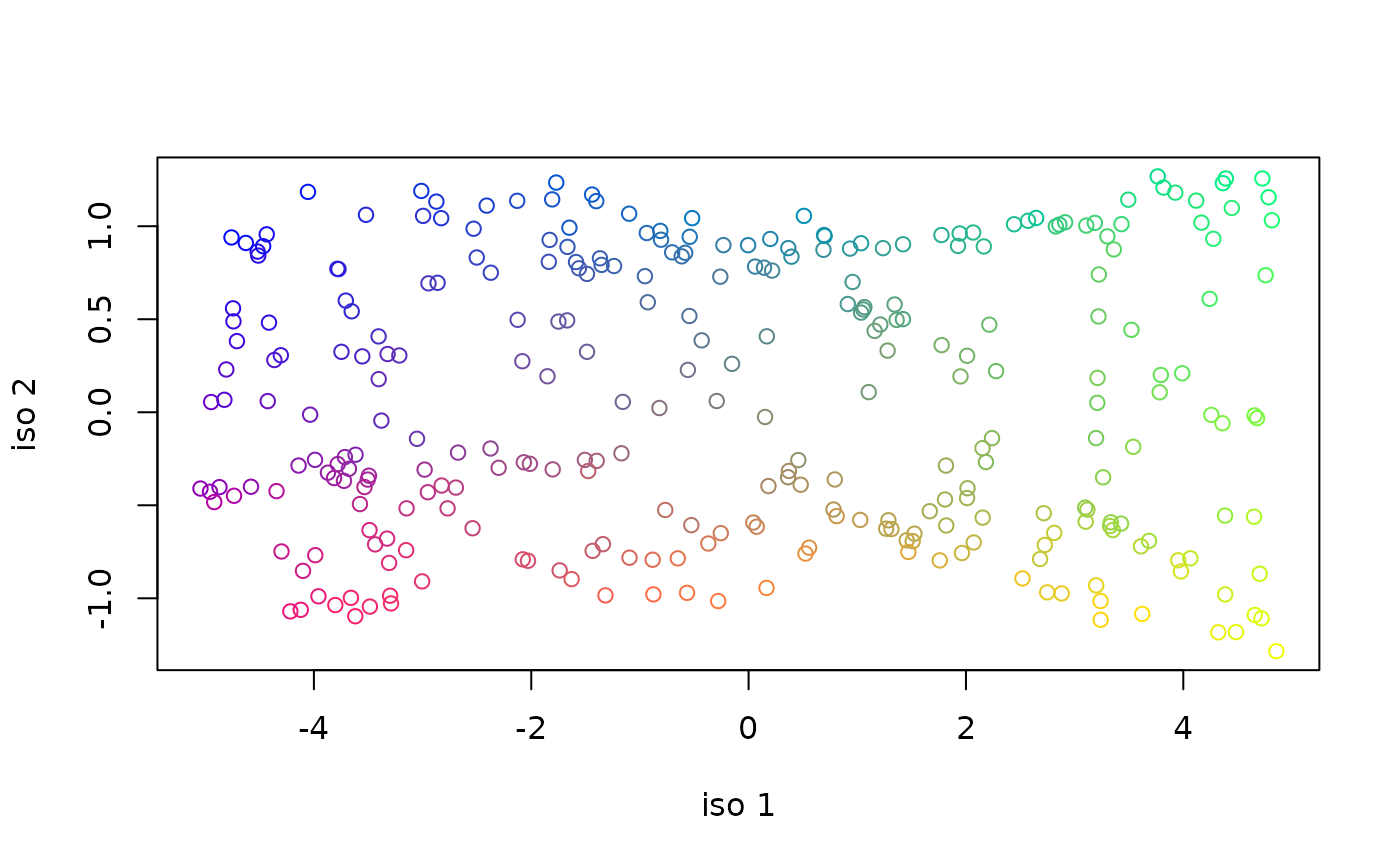
emb3 <- predict(emb2, dat[-samp])

plot(emb2, type = "2vars")
plot(emb3, type = "2vars")

}
#> 2025-04-27 07:32:14.727217: Isomap START
#> 2025-04-27 07:32:14.727647: constructing knn graph
#> 2025-04-27 07:32:14.731803: calculating geodesic distances
#> 2025-04-27 07:32:14.786848: Classical Scaling

#> 2025-04-27 07:32:14.798598: Isomap START
#> 2025-04-27 07:32:14.799355: constructing knn graph
#> 2025-04-27 07:32:14.802548: calculating geodesic distances
#> 2025-04-27 07:32:14.814834: Classical Scaling
#> 2025-04-27 07:32:14.825646: L-Isomap embed START
#> 2025-04-27 07:32:14.82734: constructing knn graph
#> 2025-04-27 07:32:14.832944: calculating geodesic distances
#> 2025-04-27 07:32:14.878304: embedding
#> 2025-04-27 07:32:14.880769: DONE

