Diffusion Maps

An S4 Class implementing Diffusion Maps

Details

Diffusion Maps uses a diffusion probability matrix to robustly approximate a manifold.

Slots

fun

A function that does the embedding and returns a dimRedResult object.

stdpars

The standard parameters for the function.

General usage

Dimensionality reduction methods are S4 Classes that either be used directly, in which case they have to be initialized and a full list with parameters has to be handed to the @fun() slot, or the method name be passed to the embed function and parameters can be given to the ..., in which case missing parameters will be replaced by the ones in the @stdpars.

Parameters

Diffusion Maps can take the following parameters:

d

a function transforming a matrix row wise into a distance matrix or dist object, e.g. dist.

ndim

The number of dimensions

eps

The epsilon parameter that determines the diffusion weight matrix from a distance matrix d, \(exp(-d^2/eps)\), if set to "auto" it will be set to the median distance to the 0.01*n nearest neighbor.

t

Time-scale parameter. The recommended value, 0, uses multiscale geometry.

delta

Sparsity cut-off for the symmetric graph Laplacian, a higher value results in more sparsity and faster calculation. The predefined value is 10^-5.

Implementation

Wraps around diffuse, see there for details. It uses the notation of Richards et al. (2009) which is slightly different from the one in the original paper (Coifman and Lafon, 2006) and there is no \(\alpha\) parameter. There is also an out-of-sample extension, see examples.

References

Richards, J.W., Freeman, P.E., Lee, A.B., Schafer, C.M., 2009. Exploiting Low-Dimensional Structure in Astronomical Spectra. ApJ 691, 32. doi:10.1088/0004-637X/691/1/32

Coifman, R.R., Lafon, S., 2006. Diffusion maps. Applied and Computational Harmonic Analysis 21, 5-30. doi:10.1016/j.acha.2006.04.006

See also

Other dimensionality reduction methods: AutoEncoder-class, DRR-class, DrL-class, FastICA-class, FruchtermanReingold-class, HLLE-class, Isomap-class, KamadaKawai-class, MDS-class, NNMF-class, PCA-class, PCA_L1-class, UMAP-class, dimRedMethod-class, dimRedMethodList(), kPCA-class, nMDS-class, tSNE-class

Examples

if(requireNamespace("diffusionMap", quietly = TRUE)) {
dat <- loadDataSet("3D S Curve", n = 300)
emb <- embed(dat, "DiffusionMaps")

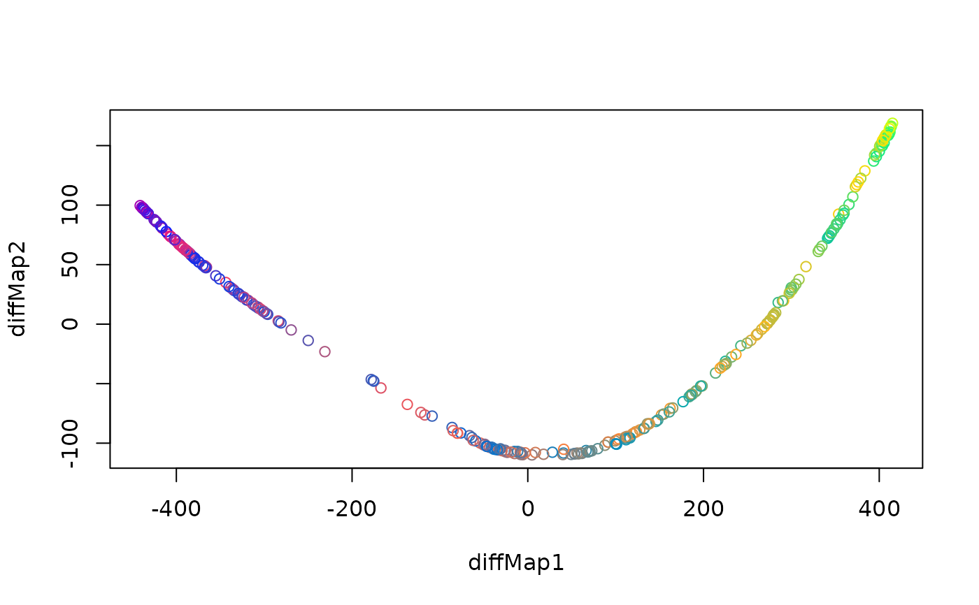
plot(emb, type = "2vars")

# predicting is possible:
samp <- sample(floor(nrow(dat) / 10))
emb2 <- embed(dat[samp])
emb3 <- predict(emb2, dat[-samp])

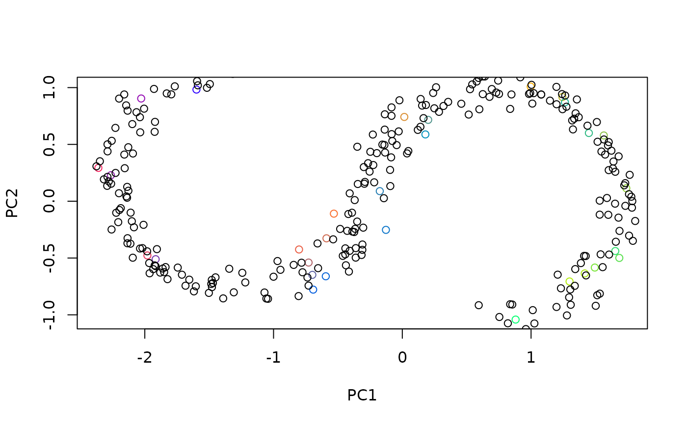
plot(emb2, type = "2vars")
points(getData(emb3))
}
#> Performing eigendecomposition
#> Computing Diffusion Coordinates
#> Elapsed time: 0.036 seconds